Ice and Climate Modeling, GPHYS/ATMS 514

Course Announcement for Winter 2001

Instructors: Cecilia Bitz and Gerard Roe

This course will cover the principles of global climate modeling from energy balance models to general circulation models. We will emphasize the application of models to study ice-sheets, snow cover, and sea ice. Topics include modern climate, climate change, Pleistocene ice ages, and snowball Earth. Students will gain hands-on experience in class periods devoted to computer-laboratory work with simple climate models, which we will provide.

We will assign approximately five homework sets. Each student will choose an additional topic and lead a class presentation on that topic. The presentation may be based on a critique of a paper or group of papers, analysis of data, and/or a simple modeling project. The project should be summarized in a brief written report. There will be no exams.

Prerequisite: GPHYS/ATMS 511 and ATMS 501 would be helpful, but are not required. No previous modeling experience needed.

Reading will be from "Paleoclimatolgy" by Crowley and North, "Ice Ages: Solving the Mystery" by Imbrie and Imbrie, handouts, and journal articles.

Please contact us if you have any questions or suggestions.

cecilia bitz, email bitz@apl.washington.edu or phone 543-1339,

or Gerard Roe, email gerard@atmos.washington.edu or phone 543-0570.

Syllabus

Lecture C/G/A   Topic
 
1-2     C     Introduction to course topics and organization
2-3,5   G     Energy balance modeling
4       G&C   Lab class on energy balance modeling
6-7     C     Basics of sea ice
8       C&G   Lab class on sea ice or ice sheet modeling
9-11    G     Ice sheet modeling, mountain glaciers and climate
11-12   G     Paleoclimate, Alternatives to and refinements of 
                Milankovitch theories
13      C     Permafrost and high latitude land surface processes
14      C     Coupled modeling
15      A     Dave Bailey: Modeling Antarctic Climate
15      C     Coupled modeling continued
16      A     Lyn Gualtieri: Interpreting data to decipher clues about
                the ice ages
16      C     Coupled modeling continued
17      A     Bonnie Light: The optics of sea ice
17      A     Ignatius Rigor: The AO and the Odden
18      A     Jennifer Kay: The Younger Dryas
18      A     Trude Storelvmo: Ice in clouds
19      A     Alison Anderse: The climate of Mars
19      A     Llyd Wells: Snowball earth
20      C&G   Wrap up

Following is a brief description of the two lab class projects we will give for this course. You may download a tarfile with all the matlab scripts necessary to run the models with the graphical user interfaces. The tarfile includes the assignments we will give to guide the user through a series of excercises with the models. These are pdf files lab1.pdf and lab2.pdf. In the first lab class you will use a one-dimensional energy balance model of the type described in the early papers by Budyko, Sellers, and North. The solar forcing is seasonally averaged and the model is run each time to equilibrium. The model is coded in matlab but it is run using a graphical user interface.

Annual Mean EBM GUI

A screen shot of the matlab GUI is shown to the left. You can easily alter the overall amplitude of the meridional heat transport D, the amplitude of the solar constant relative to present day measurements Q/Qo, and coefficient of the linearized outgoing longwave radiation A+BT. You can also turn off the albedo feedback so the model uses an albedo prescribed to be identical to that from the model run with the default parameter set. The meridional heat transport can approximate the affect of the Hadley Circulation as suggested by Lindzen and Farrell, 1977. Normally the initial temperature profile is consistent with a non-glaciated climate. Pressing the cold start button will change the initial conditions so the initial profile approximates a snowball earth.

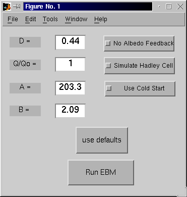
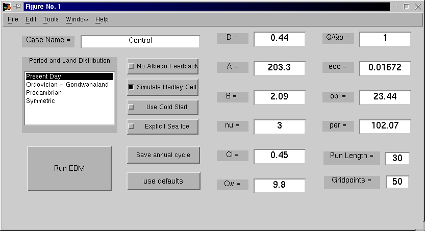
The second lab uses a seasonally varying one-dimensional energy balance model based on the work of North and Coakley, 1979, but we added an explicit sea ice model. The screen shot of the model GUI shows the versatility of the model and the lab excersices contains a description of the model.

If the model misbehaves such as graphics appear in the background of the GUI, avoid clicking on any graphics windows while the model is running. Matlab is less than robust and we are less than pros at programming GUIs.

We recommend reading North and Coakley, 1979: Differences between Seasonal and Mean Annual Energy Balance Model Calculations of Climate and Climate Sensitivity. Journal of the Atmospheric Sciences: Vol. 36, No. 7, pp. 1189-1204, for the January 11 lab class on energy balance modeling (EBM). In particular, pay special attention to Equations 13-18 in section 4. Read sections 5-10 for physical insights and to gain an appreciation for the utility of EBMs. Familiarity with the details of the truncated spectral solutions (mode-solutions) is not necessary. Don't get bogged down in the math, unless you enjoy it.

Another good source of reading about EBMs is chapter 2 of "Dynamics in Atmospheric Physics" by Richard Lindzen.

Last modified: Tue Feb 13 18:19:27 PST 2001